Physikalische Simulationen

Armas Scharpegge

Ratsgymnasium Bielefeld

DPG Schülertagung 2023

Inhalt

Warum Simulationen?
Methodik
Punktmasse mit Kraft
Gravitations-Simulation
Wellen-Simulation
Fazit

Simulationen

Vorhersagen über physikalische System
- Sonnensystem, Asteroide
- Verhalten von Materialien und Bauteilen
- Automatisierung von Tests
- Vergleich mit experimentellen Daten
- Virtuelle Welten (Videospiele, Filme)

Methodik

Modellierung des Systems
(Numerische) Lösung der Modellierung

Beide Schritte lassen sich auf viele verschiedene Weisen lösen!

Vektoren

Vektor

Größe in mehreren Dimensionen
- 2D: \(x\) und \(y\) Koordinate
- 3D: \(x\), \(y\) und \(z\) Koordinate
Rechenoperationen beziehen sich auf alle Dimensionen

Addition 2D

\begin{align*} \begin{pmatrix} \mathbf{a}_x \\ \mathbf{a}_y \end{pmatrix} + \begin{pmatrix} \mathbf{b}_x \\ \mathbf{b}_y \end{pmatrix} = \begin{pmatrix} \mathbf{a}_x + \mathbf{b}_x \\ \mathbf{a}_y + \mathbf{b}_y \end{pmatrix} \end{align*}

Addition 3D

\begin{align*} \begin{pmatrix} \mathbf{a}_x \\ \mathbf{a}_y \\ \mathbf{a}_z \end{pmatrix} + \begin{pmatrix} \mathbf{b}_x \\ \mathbf{b}_y \\ \mathbf{b}_z \end{pmatrix} = \begin{pmatrix} \mathbf{a}_x + \mathbf{b}_x \\ \mathbf{a}_y + \mathbf{b}_y \\ \mathbf{a}_z + \mathbf{b}_z \end{pmatrix} \end{align*}

Skalarmultiplikation

\begin{align*} k \begin{pmatrix} \mathbf{a}_x \\ \mathbf{a}_y \end{pmatrix} = \begin{pmatrix} k\mathbf{a}_x \\ k\mathbf{a}_y \end{pmatrix} \end{align*}

Ableitung

\begin{align*} f'(x) & = \frac{\mathrm{d}f}{\mathrm{d}x} \\ & = \lim_{h\rightarrow 0} \frac{f(x+h) - f(x)}{h} \end{align*}

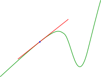
Steigung (der Tangente) an Stelle \(x\)
Wieviel verändert sich \(f\) pro \(x\) (genau an der Stelle \(x\))?

Ableitung

Punktmasse

Notation

\begin{align*} &\text{Position} & \mathbf{x}(t) & = \begin{pmatrix}\mathbf{x}_x \\ \mathbf{x}_y \\ \mathbf{x}_z \end{pmatrix} \\ &\text{Geschwindigkeit} & \mathbf{\dot{x}}(t) & = \frac{\mathrm{d}\mathbf{x}}{\mathrm{d}t} = \mathbf{v} \\ &\text{Beschleunigung} & \mathbf{\ddot{x}}(t) & = \frac{\mathrm{d}^2\mathbf{x}}{\mathrm{d}t^2} = \mathbf{a} \\ \end{align*}

Newtons Gesetze

Ein kräftefreier Körper bleibt in Ruhe oder bewegt sich geradlinig mit konstanter Geschwindigkeit.
\(\mathbf{F} = m\mathbf{\ddot{x}} = m\mathbf{a}\)
Kraft gleich Gegenkraft: Eine Kraft von Körper A auf Körper B geht immer mit einer gleich großen, aber entgegen gerichteten Kraft von Körper B auf Körper A einher.

Differentialgleichung

\begin{align*} \mathbf{x}(0) & = \mathbf{x}_0 \\ \mathbf{\dot{x}}(0) & = \mathbf{v}_0 \\ \mathbf{\ddot{x}}(t) & = \frac{\mathbf{F}(t)}{m} = \mathbf{a}(t) \end{align*}

Lösung

Wenn \(\mathbf{\ddot{x}}(t)\) nur von \(t\), aber nicht von \(\mathbf{x}(t)\) und \(\mathbf{\dot{x}}(t)\) abhängig ist:

\begin{align*} \mathbf{\dot{x}}(t) & = \mathbf{v}_0 + \int_{0}^{t} \mathbf{\ddot{x}}(x) \, dx \\ \mathbf{x}(t) & = \mathbf{x}_0 + \int_{0}^{t} \mathbf{\dot{x}}(x) \, dx \\ & = \mathbf{x}_0 + \mathbf{v}_0 t + \int_{0}^{t} \int_{0}^{x} \mathbf{\ddot{x}}(y) \, dy \, dx \\ \end{align*}

Konstante Kraft

\begin{align*} \mathbf{x}(t) & = \mathbf{x}_0 + \mathbf{v}_0 t + \int_{0}^{t} \int_{0}^{x} \mathbf{a} \, dy \, dx \\ & = \mathbf{x}_0 + \mathbf{v}_0 t + \int_0^t \mathbf{a} x \, dx \\ & = \mathbf{x}_0 + \mathbf{v}_0 t + \frac{1}{2} \mathbf{a} t^2 \end{align*}

\begin{align*} \mathbf{\dot{x}}(t) = \mathbf{v}_0 + \mathbf{a} t \end{align*}

🎉

Umsetzung

function getAnalyticPosition(x0, v0, a, t)
{
    // x = x0 + v0 * t + 1/2 * a * t^2
    return x0.add(v0.mul(t)).add(a.mul(0.5 * t * t));
}

function getAnalyticVelocity(v0, a, t)
{
    // v = v0 + a * t
    return v0.add(a.mul(t));
}

Schräger Wurf

var initialPos = new Vector2(0.5, 2);
var initialVelocity = new Vector2(8, 4);
var gravityVec = new Vector2(0.0, -9.81);

Mit steigendem currentTime:

curPos = getAnalyticPosition(initialPos, initialVelocity,
                             gravityVec, currentTime);
curVel = getAnalyticVelocity(initialVelocity, gravityVec,
                             currentTime);

Demo

Gravitations-Simulation

Modellierung

Für \(n\) Partikel \(i=1,2, \dots, n\):

\begin{align*} \mathbf{x}_i(0) & = \mathbf{x}_{i,0} \\ \mathbf{\dot{x}}_i(0) & = \mathbf{v}_{i,0} \\ \mathbf{\ddot{x}}_i(t) & = \frac{\mathbf{F}_{i}}{m} \\ \end{align*}

Modellierung

\begin{align*} F & = \gamma \frac{m_1m_2}{r^2} \end{align*}

\begin{align*} \mathbf{F}_{i,j} & = \gamma \frac{m_i m_j}{\lVert \mathbf{r}_{i,j} \rVert^2} \mathbf{\hat{r}}_{i,j} \\ \mathbf{r}_{i,j} & = \mathbf{x}_j - \mathbf{x}_i \\ \mathbf{\hat{r}}_{i,j} & = \frac{\mathbf{r}_{i,j}}{\lVert \mathbf{r}_{i,j} \rVert} \end{align*}

Modellierung

\begin{align*} \mathbf{F}_i & = \sum_{j \ne i} \mathbf{F}_{i,j} \\ & = \mathbf{F}_{i,1} + \mathbf{F}_{i,2} + \cdots + \mathbf{F}_{i,i-1} + \mathbf{F}_{i,i+1} + \cdots + \mathbf{F}_{i,n} \end{align*}

Analytische Lösung?

Integrieren geht nicht! (\(\mathbf{\ddot{x}}(t)\) hängt von \(\mathbf{x}(t)\) ab)

Selbst für \(n=3\) ist keine allgemeine Lösung durch Elementarfunktionen bekannt (Three-body problem) [1].

Lösung: Numerische Integration

Numerische Integration

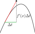
Explizites Eulerverfahren [2]

\begin{align*} \mathbf{x}_n & \approx \mathbf{x}(n \Delta t) \\ \mathbf{\dot{x}}_{n+1} & = \mathbf{\dot{x}}_n + \Delta t \mathbf{\ddot{x}}_n \\ \mathbf{x}_{n+1} & = \mathbf{x}_n + \Delta t \mathbf{\dot{x}}_{n} \end{align*}

Symplektisches Eulerverfahren [3]

\(\Rightarrow\) bessere Energieerhaltung

Code

class EulerParticle2 {
    constructor(m = 1.0,
                x = new Vector2(0.0, 0.0),
                v = new Vector2(0.0, 0.0)) {
        this.m = m;
        this.x = x.clone();
        this.v = v.clone();
    }

    // ...
}

Code

    step(F, dt) {
        // v' = v + F/m * dt
        this.v = this.v.add(F.mul(dt / this.m));
        // x' = x + v' * dt
        this.x = this.x.add(this.v.mul(dt));
    }

Code

    unstep(F, dt) {
        // x = x' - v' * dt
        this.x = this.x.sub(this.v.mul(dt));
        // v = v' - F/m * dt
        this.v = this.v.sub(F.mul(dt / this.m));
    }

Code

var GRAV_CONSTANT = 6.674e-11;

function calcForce(x1, m1, x2, m2) {
    var r = x2.sub(x1);
    var rLen2 = r.len2();
    var rLen = r.len();
    return r.mul(GRAV_CONSTANT * m1 * m2 / rLen2 / rLen);
}

Code

function simulateForward(deltaTime, numSubsteps) {
    currentTime += deltaTime;
    var dt = deltaTime / numSubsteps;

    for (var substep = 0; substep < numSubsteps; substep++) {
        // ...
    }
    for (var i = 0; i < particles.length; i++) {
        lastParticlePos[i].push(particles[i].x.clone());
    }
}

Code

var particle_forces = [];
for (var i = 0; i < particles.length; i++)
    particle_forces.push(new Vector2(0.0, 0.0));
for (var i = 0; i < particles.length; i++) {
    for (var j = i+1; j < particles.length; j++) {
        var F = calcForce(particles[i].x, particles[i].m,
                          particles[j].x, particles[j].m);
        particle_forces[i] = particle_forces[i].add(F);
        particle_forces[j] = particle_forces[j].add(F.neg());
    }
    particles[i].step(particle_forces[i], dt);
}

Demo

Wellen-Simulation

1D Wellengleichung

\begin{align*} \partial_{tt} u(t,x) & = c^2 \partial_{xx} u(t,x) \\ \\ u(t,x) & : \text{ Auslenkung an Position } x \text{ zur Zeit } t \\ c & : \text{ Ausbreitungsgeschwindigkeit} \\ \end{align*}

Partielle Ableitung

\begin{align*} \partial_t u & = \lim_{h \rightarrow 0} \frac{u(t+h,x) - u(t,x)}{h} \\ \end{align*}

Partielle Ableitung

\begin{align*} u(t,x) & = x^2 + e^{xt} \\ \partial_t u & = x e^{xt} \\ \partial_{tt} u & = x^2 e^{xt} \\ \partial_{xx} u & = 2 + t^2 e^{xt} \end{align*}

2D Wellengleichung

\begin{align*} \partial_{tt} u & = c^2 \left( \partial_{xx} u + \partial_{yy} u \right)\\ \\ u(t,x,y) & : \text{ Auslenkung an Position } (x,y) \text{ zur Zeit } t \\ c & : \text{ Ausbreitungsgeschwindigkeit} \\ \end{align*}

Voraussetzungen

Initial conditions: Anfangszustand
Boundary conditions: Dauerhafte Grenzbedingungen
- nicht unbedingt nur an den Rändern (Wände im Raum)

Analytische Lösung?

nur ohne / mit einfachen Grenzbedingungen

\(\Rightarrow\) numerische Lösung

Diskretisierung

\begin{align*} t_n & = t_0 + n\Delta t \\ u_{n,i,j} & = u(t_n, i \Delta x, j \Delta x) \end{align*}

Geometrie

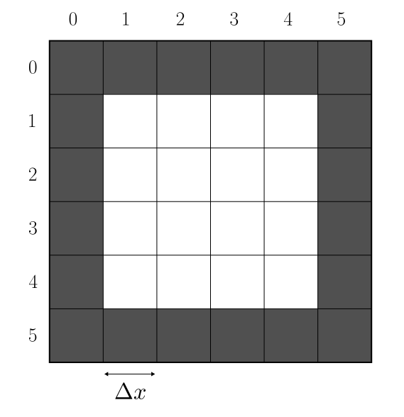
Finite Difference Method [4]

Lösungsmethode für partielle Differentialgleichungen
Diskretisierung der Variablen (\(t\) und \(u\))
Diskretisierung der Ableitungen
Lösung der resultierenden normalen Gleichung

Central Difference Scheme

\begin{align*} \partial_{tt} u_{n,i,j} & \approx \frac{\frac{u_{\mathbf{\color{red} {n+1}},i,j} - u_{\mathbf{\color{red}{n}},i,j}}{\Delta t} - \frac{u_{\mathbf{\color{red}{n}},i,j} - u_{\mathbf{\color{red}{n-1}},i,j}}{\Delta t} }{\Delta t} \\ & = \frac{\left(u_{\mathbf{\color{red}{n+1}},i,j} - u_{\mathbf{\color{red}{n}},i,j} \right) - \left(u_{\mathbf{\color{red}{n}},i,j} - u_{\mathbf{\color{red}{n-1}},i,j}\right) }{\Delta t^2} \\ & = \frac{u_{\mathbf{\color{red}{n+1}},i,j} - 2u_{\mathbf{\color{red}{n}},i,j} + u_{\mathbf{\color{red}{n-1}},i,j}}{\Delta t^2} \\ \end{align*}

Central Difference Scheme

\begin{align*} \partial_{\mathbf{\color{red}{tt}}} u_{n,i,j} & \approx \frac{u_{\mathbf{\color{red}{n+1}},i,j} - 2u_{\mathbf{\color{red}{n}},i,j} + u_{\mathbf{\color{red}{n-1}},i,j}}{\Delta t^2} \\ \partial_{\mathbf{\color{red}{xx}}} u_{n,i,j} & \approx \frac{u_{n,\mathbf{\color{red}{i+1}},j} - 2u_{n,\mathbf{\color{red}{i}},j} + u_{n,\mathbf{\color{red}{i-1}},j}}{\Delta x^2} \\ \partial_{\mathbf{\color{red}{yy}}} u_{n,i,j} & \approx \frac{u_{n,i,\mathbf{\color{red}{j+1}}} - 2u_{n,i,\mathbf{\color{red}{j}}} + u_{n,i,\mathbf{\color{red}{j-1}}}}{\Delta x^2} \\ \end{align*}

Lösen

Gesuchst ist \(u_{\mathbf{\color{red}{n+1}},i,j}\).

Gesamtgleichung

Mit \(d_{\mathbf{\color{red}i}} = u_{n,\mathbf{\color{red}{i+1}},j} - 2u_{n,\mathbf{\color{red}i},j} + u_{n,\mathbf{\color{red}{i-1}},j}\) etc.:

\begin{align*} \partial_{tt} u & = c^2 \left( \partial_{xx} u + \partial_{yy} u \right) \\ \Rightarrow \frac{u_{\mathbf{\color{red}{n+1}},i,j} - 2u_{n,i,j} + u_{\mathbf{\color{red}{n-1}},i,j}}{\Delta t^2} & = c^2 \left( \frac{d_\mathbf{\color{red}{i}}}{\Delta x^2} + \frac{d_\mathbf{\color{red}{j}}}{\Delta x^2} \right) \\ \Leftrightarrow u_{\mathbf{\color{red}{n+1}},i,j} = 2u_{n,i,j} - u_{\mathbf{\color{red}{n-1}},i,j} & + \frac{c^2\Delta t^2}{\Delta x^2} \left(d_\mathbf{\color{red}{i}} + d_\mathbf{\color{red}{j}}\right) \end{align*}

Gesamtgleichung

\begin{align*} s & = u_{n,\mathbf{\color{red}{i+1}},j} + u_{n,i,\mathbf{\color{red}{j+1}}} + u_{n,\mathbf{\color{red}{i-1}},j} + u_{n,\mathbf{\color{red}{j-1}}} \\ k & = \frac{c^2\Delta t^2}{\Delta x^2} \\ u_{\mathbf{\color{red}{n+1}},i,j} & = \left(2 - k\right)u_{n,i,j} + k s - u_{\mathbf{\color{red}{n-1}},i,j} \end{align*}

\(\Rightarrow\) Neuer Zustand kann durch aktuellen + vorherigen Zustand berechnet werden (3 Buffer).

Initial conditions

beliebige Anfangszustände für \(u_{0,i,j}\) und \(u_{-1,i,j}\)
z.B. Kreiswelle oder Punkt

Boundary conditions

\(u_{n,i-1,j}\) am linken Rand nicht gegeben (usw.)
- Extra-Schicht an allen Seiten, die nicht normal simuliert wird

Geometrie

Dirichlet condition

fester Wert (\(0\)) an den Grenzen
festes Ende
Reflexion mit Vorzeichenwechsel

Wände

eine Zelle kann als Wand markiert werden
z.B. Dirichlet condition
- Zelle hat immer Wert \(0\)

Quellen

eine Zelle oszilliert andauernd
- Dirichlet condition

\begin{align*} u_{t,i,j} & = A_0 \cos \left( \omega t \right) \end{align*}

Absorbing boundary condition

keine Reflexion der Welle
Perfectly matched layer: Spezielle Dämpfung an den Rändern [5]

nicht so einfach =¯\_(ツ)_/¯=

Implementation

class Buffers {
    constructor(width, height) {
        this.b = [
            new Float32Array(width * height),
            new Float32Array(width * height),
            new Float32Array(width * height)
        ];
        this.prevIdx = 0;
    }
}

Triple Buffer

class Buffers {
    prev() {
        return this.b[this.previdx];
    }
    cur() {
        return this.b[(this.previdx + 1) % 3];
    }
    next() {
        return this.b[(this.previdx + 2) % 3];
    }
}

Triple Buffer

class Buffers {
    step() {
        this.prevIdx = (this.prevIdx + 1) % 3;
    }
}

WaveSim Init

class WaveSim {
    constructor(width, height, dt, dx, c) {
        this.w = width; this.h = height; this.dt = dt;
        this.dx = dx; this.c = c;

        this.k = this.c * this.dt / this.dx;
        this.k = this.k * this.k;
        this.time = 0.0;
        this.b = new Buffers(width+2, height+2);
    }
}

WaveSim Reset

class WaveSim {
    reset() {
        this.time = 0.0;
        this.b.prev().fill(0.0);
        this.b.cur().fill(0.0);
        this.b.next().fill(0.0);
        this.setBoundary();
    }
}

WaveSim Step

class WaveSim {
    step() {
        for (var y = 1; y < this.h+1; y++) {
            for (var x = 1; x < this.w+1; x++) {
                // calc
            }
        }
        this.b.step();
        this.setBoundary();
        this.time += this.dt;
    }
}

WaveSim Calc

this.b.next()[y * (this.w + 2) + x] =
    (2 - 4 * this.k) * this.b.cur()[y * (this.w + 2) + x]
    - this.b.prev()[y * (this.w + 2) + x]
    + this.k * (
        this.b.cur()[y * (this.w + 2) + x + 1]
            + this.b.cur()[y * (this.w + 2) + x - 1]
            + this.b.cur()[(y + 1) * (this.w + 2) + x]
            + this.b.cur()[(y - 1) * (this.w + 2) + x]
    );

WaveSim Boundary

function slitBoundary(sourceX, sourceY, slitSize,
    slitPadding, slitMiddle, slitPos, m, numSlits) {
    return function() {
        this.b.cur()[(sourceY + 1) * (this.w + 2)
            + sourceX + 1] = Math.cos(this.time * 10);

        // set all wall cells to 0
        // ...
    }
}

Demo

Extra

Simulationen von Nils Berglund auf YouTube
- Tutorial: How to simulate the wave equation [6]
Ten Minute Physics von Matthias Müller [7]

Fazit

(partielle) Differenzialgleichungen
meist nur numerische Lösung möglich
- Diskretisierung von Zeit und Raum
für bekannte Kraft: numerische Integration

Einfach mal ausprobieren!

Quellen

[1]

Wikipedia contributors, “Three-body problem –- Wikipedia, the free encyclopedia.” 2023. Available: https://en.wikipedia.org/wiki/Three-body_problem

[2]

Wikipedia contributors, “Euler method –- Wikipedia, the free encyclopedia.” 2023. Available: https://en.wikipedia.org/wiki/Euler_method

[3]

Wikipedia contributors, “Semi-implicit euler method –- Wikipedia, the free encyclopedia.” 2023. Available: https://en.wikipedia.org/wiki/Semi-implicit_Euler_method

[4]

Wikipedia contributors, “Finite difference method –- Wikipedia, the free encyclopedia.” 2023. Available: https://en.wikipedia.org/wiki/Finite_difference_method

[5]

Wikipedia contributors, “Perfectly matched layer –- Wikipedia, the free encyclopedia.” 2023. Available: https://en.wikipedia.org/wiki/Perfectly_matched_layer

[6]

Nils Berglund, Ed., Tutorial: How to simulate the wave equation, (Jul. 08, 2023). Accessed: Jul. 22, 2023. [Online]. Available: https://www.youtube.com/watch?v=pN-gi_omIVE

[7]

M. Müller, “Ten Minute Physics.” 2023. Available: https://matthias-research.github.io/pages/tenMinutePhysics/index.html

Dateien

https://ascharpegge.codeberg.page/dpg23

Lizenzen

Code: Apache-2.0
Inhalte: CC-BY-SA-4.0
QR-Code: CC0-1.0